SMOS has opened a new field of research and application (one more!)
Observing sea surface state under a Hurricane
By Joe Tenerelli (CLS Brest)
It is well known that the L-band brightness temperatures measured by a downward looking radiometer such as that on board SMOS are significantly influenced by a number of radiation sources. Among the most important sources of L-band brightness over the ocean are:
1) flat surface emission (with order of magnitude 100 K);2) Atmospheric emission (on the order of 5 K including reflected downwelling and upwelling);3) scattered galactic radiation incident at the surface (order of magnitude 10 K);4) excess emission associated with wind-driven surface roughness (order of magnitude 10 K).
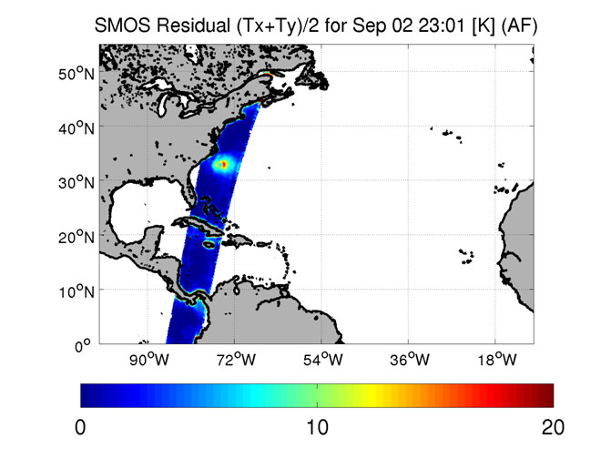
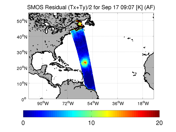
By formulating a forward model of scene brightness for each of these sources, we can remove all but one of these contributions in order to reveal individual sources. For example, by removing all but the flat surface emission and by linearizing the salinity dependence about some reference value, we can retrieve deviations of surface salinity from that reference.Similarly, by removing all but the scattered galactic noise contribution and projecting the remaining brightness onto the celestial sphere, we can obtain maps of scattered galactic noise as a function of surface wind speed (see an earlier post for results of this exercise).Analogously, we can remove all but the rough surface emission to reveal the impact of roughness on the brightness temperatures at the radiometer. When we do this, we find a significant residual signal that continues to steadily increase up through hurricane force winds.Below are two maps showing the first Stokes parameter (divided by two) of this residual roughness brightness. The residuals have been averaged over the dwell lines formed as the satellite passes over fixed points on earth. To the left we see this residual for Hurricane Earl at 2300 UTC 02 September, when it was a category 3 hurricane with maximum surface wind speed of 100 kt (about 51 m/s or 115 miles/hour). The residual first Stokes parameter (divided by two) reaches nearly 20 K to the right of the storm, which is a very significant signal and well above the per-dwell line noise level.Similarly, the residual first Stokes (Tx+Ty)/2 for hurricane Igor near 0900 UTC 17 September is shown below and to the right, when it was a category 3 hurricane with maximum sustained surface wind speed of near 110 kt (about 55 m/s or 125 miles/hour). As with Earl, the roughness residual (Tx+Ty)/2 reaches nearly 20 K.
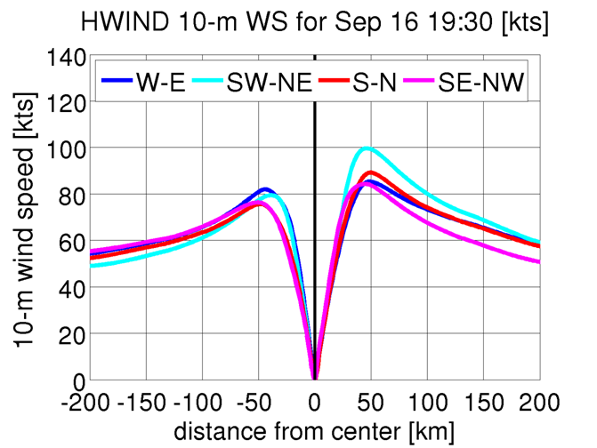
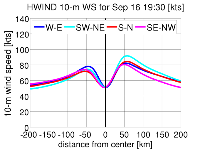
Since the SMOS interferometric radiometer, only samples a limited range of spatial frequencies, the spatial resolution of reconstructed brightness temperature maps is limited and features with scales less than about 50 km are strongly smoothed. Therefore, in order to compare SMOS roughness residual brightness temperatures to the HWIND wind fields we applied an average SMOS synthetic beam weighting function to the HWIND wind field in order to derive a smoothed wind field. Below we show various cross sections through the unsmoothed (left) and smoothed (right) HWIND analysis for 1930 UTC 16 September. The large impact of this smoothing is evident: Compared to the unsmooth wind field, the radius of maximum wind speed increases by a few kilometers, the maximum wind speed decreases from 100 kt to about 90 kt, and the minimum surface wind speed at the storm center increases to about 50 kt.Strictly speaking, the problem of relating synthetic beam smoothed brightness temperatures to ‘smoothed’ wind fields is ill-posed, since, without any assumptions, one can generally find multiple distributions of unsmoothed wind fields that yield different smoothed brightness temperature fields for the same smoothed wind field. However, to the extent that the roughness residual brightness temperature varies linearly with wind speed, we can justifiably derive a ‘smoothed’ model by relating a smoothed wind field to synthetic beam averaged brightness temperature field.
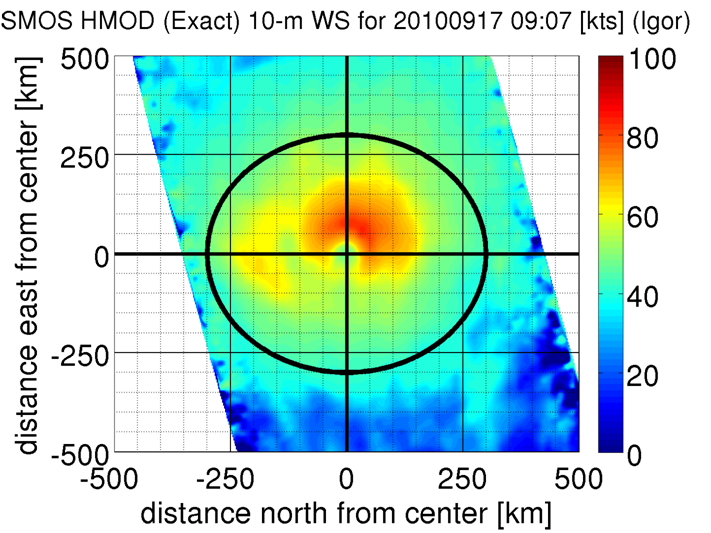
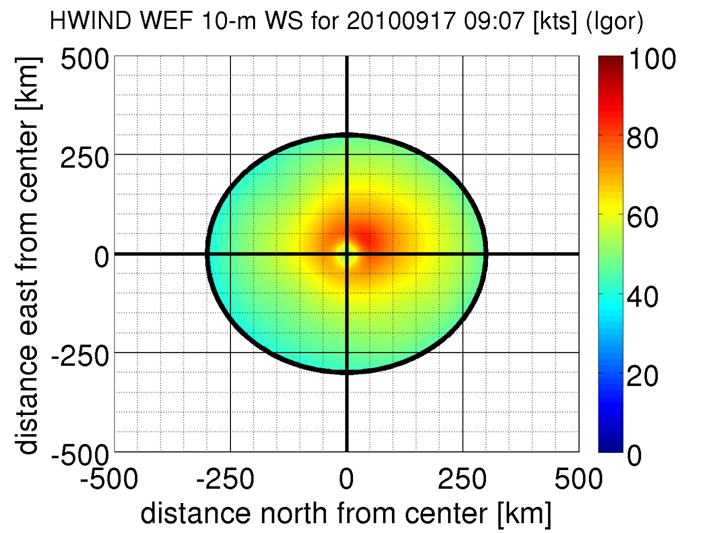
Examining more closely the roughness residual first Stokes parameter for the hurricane Igor overpass on 17 September, we see that the pattern of L-band brightness residual closely resembles that of the near-surface wind field derived by the NOAA AOML Hurricane Research Division (HRD) based in Miami, Florida. In the figure below and to the left, we show the residual first Stokes parameter from SMOS in a cartesian coordinate system with origin at the storm center. To the right we show the HRD surface wind field analysis, derived using their HWIND analysis system, for 1930 UTC 16 September. In this case (but not always) the HWIND analysis field incorporates (among many other sources of data) surface wind speeds derived (along with rain rate) from a C-band Stepped Frequency Microwave Radiometer (SFMR). For excellent descriptions of the wind and rain retrieval algorithms for the SFMR see the papers of Uhlhorn et al. and Jiang et al., Monthly Weather Review 2003, 2006, and 2007. Other sources of wind information for this analysis include GPS sondes, an ASCAT pass, and a buoy time series.
To derive an empirical relationship between residual SMOS total power and surface wind speed we use two HWIND surface wind fields derived for 1930 UTC on September 16 and 17. Unfortunately, the analyses are separated by a day with the SMOS overpass occurring midway between them, and in this time period the storm was beginning to weaken. To arrive at a very rough approximate wind field for deriving a model we take the average of the two HWIND analyses and we recognize that some error may be introduced in this averaging.
In deriving the model, we will assume that all of the residual brightness is related to roughness and that none is related to precipitation. At L-band, emission and attenuation from precipitation if much lower than at higher frequencies; nevertheless, it is clear that the brightness temperatures may increase by several kelvin in the vicinity of rainband, and research involving collocated passive and active data at higher frequencies is required in order to address this issue.
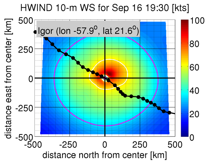
The approach we take here is to simply find the function that maps the SMOS brightness temperatures into a ‘wind field’ with a probability distribution that matches that of the temporally averaged and spatially smoothed wind field obtained from the two HWIND analyses. This matching considers only winds within 300 km of storm center and the domain is shown in the third figure above.
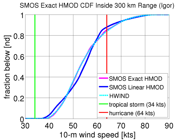
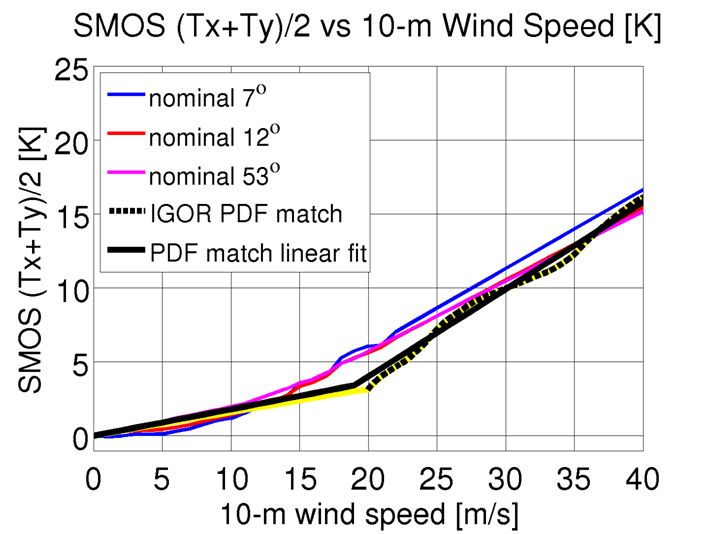
Below and to the left we show the CDFs obtained from the averaged HWIND analysis and those obtained from two SMOS empirical models. One using the exact PDF match and the other using a linear fit to the model derived from the PDF match. Also shown are the minimum wind speeds for tropical storms and hurricanes.
Below and to the right we show the roughness residual first Stokes parameter (divided by two) as a function of wind speed for both the exact (dashed black) and linear (solid black) PDF matching models. We also show linear extrapolations of an empirical model derived from SMOS data for wind speeds below about 23 m/s. As the hurricane model is based on dwell line averaged brightness, no direct comparisn can be made between the hurricane model and the lower wind speed model, but there is significant discrepancy between the models for all incidence angles which evidence of the special nature of sea states within hurricanes.
Below we compare the wind field derived using the hurricane L-band wind speed model (left) to the SMOS-smoothed wind field from the time-averaged averaged HWIND analysis (right).
By construction, the SMOS wind field captures the maximum wind speed, but the spatial structures in the two wind fields are somewhat different. First of all, the asymmetry across track is larger in the SMOS wind field than in the HWIND analysis, and this is probably related to variability in sea states for a given surface wind speed.
Secondly, a band of high wind speed to the SW of storm center is evident in the SMOS wind field, and this is likely associated with a rainband that is evident in higher frequency brightness temperature maps from an AMSR overpass.
Despite these discrepancies, it is clear that SMOS can capture the essential features of strong tropical cyclones, but to obtain a useful product more work is required to understand the relations between wind speed and sea state and the associated impact on L-band brightness temperature.