![]() =>
=>![]() « Winter is coming » ― George R.R. Martin, A Game of Thrones As Christmas holidays are approaching you might want to know if there is snow in your favorite spot of ski touring? A good knowledge of the snow cover variability is important – not only to plan your next week-end, but also because the snow is a key water resource in many regions, including here in south west France.
« Winter is coming » ― George R.R. Martin, A Game of Thrones As Christmas holidays are approaching you might want to know if there is snow in your favorite spot of ski touring? A good knowledge of the snow cover variability is important – not only to plan your next week-end, but also because the snow is a key water resource in many regions, including here in south west France.
The winter snowpack in the Pyrenees is like a natural water reservoir, releasing meltwater runoff during the spring, when the crops in the cultivated lowlands need to be irrigated. The snow melt is also extensively used for hydropower production. We are developing a snow cover product from Landsat-8 and Sentinel-2 data to provide the snow presence or absence at 20 m resolution every 5 days. The algorithm is simple because the snow surface is quite straightforward to detect from high resolution optical imagery. A challenge is typically to avoid the confusion between the snow cover and the clouds. Here the job was made easy since we take as input the level 2A product so we can use the cloud mask from the MAJA algorithm as a prior information. Another great advantage of the level 2A product is that it provides slope-corrected surface reflectances. Did I tell you that mountain regions are quite sloping? The slope correction enables to use the same detection thresholds in south-facing and north-facing slopes. Actually the main unresolved issue is the obstruction of the ground surface by the forest canopy, which can hinder the snow detection in evergreen forest areas. Unfortunately MAJA does not yet provide bottom of canopy reflectances…

The snow detection is based on the Normalized Difference Snow Index (NDSI): $$ \textrm{NDSI} = \frac{\rho_\textrm{{Green}}-\rho_\textrm{{MIR}}}{\rho_\textrm{{Green}}+\rho_\textrm{{MIR}}} $$ which was introduced long time ago by Jeff Dozier (Rem. Sens. Env., 1989) for Landsat TM. Here $$ \rho$$ is the surface reflectance. It also works for SPOT4/5, Landsat-8 and Sentinel-2 images since a shortwave infrared band near 1.6 µm is available. The NDSI is based on the fact that only snow surfaces are very bright in the visible but dark in the shortwave infrared. Some lakes may also have a high NDSI value so we add a criterion on the red reflectance to remove these.
Overview of the algorithm
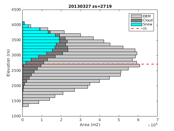
We want a robust and efficient algorithm to process large mountain regions with a reasonable computation cost. Since the snow cover extent is largely controlled by the elevation we incorporated a digital elevation model in the input data to avoid false positive in the low elevation areas and false negative in the high elevation areas. A first pass of snow detection is performed with strict thresholds on the NDSI and red reflectance values ($$N_1=0.4, R_1=0.2$$) in order to retrieve a set of pixels for which we have a very high confidence that they are well classified as snow. A pixel is marked as snow covered if: $$ \textrm{snow}_1 = \textrm{cloud}_1 \textrm{ is false and } \textrm{NDSI} \gt N_1 \textrm{ and } \rho_\textrm{Red} > R_1 $$ (Pass 1) However, we do not take the original L2A cloud mask as input $$ \textrm{cloud}_1$$ here because it is processed at a coarser resolution, very conservative and much useful information for snow cover mapping is lost. We allow the reclassification of some cloud pixels in snow or no-snow only if they have a rather low reflectance. We select only these potentially « dark clouds » because the NDSI test is robust to the snow/cloud confusion in this case. The cloud flag is removed for these pixels unless they were flagged as a cloud shadow. $$\textrm{cloud}_1 = (\textrm{cloud}_{L2A} \textrm{ and } \rho_\textrm{Red}>R_c) \textrm{ or } \textrm{« cloud shadow » is true} $$ Then we estimate the lowest elevation of the snow cover in the image ($$Z_S$$) using the SRTM digital elevation model.

Knowing that above the minimum altitude, the probability to have snow is higher, we perform another pass for the pixels located above the snowline elevation $$Z_S$$, with different threshold values ($$N_2=0.15, R_2=0.12$$): $$ \textrm{snow}_2 = Z>Z_S \textrm{ and cloud}_1 \textrm{ is false and } \textrm{NDSI} \gt N_2 \textrm{ and } \rho_\textrm{Red} > R_2 $$ (Pass 2) The final snow mask is the union of $$\textrm{snow}_1$$ and $$\textrm{snow}_2.$$ Note that some pixels originally marked as cloud in the L2A mask will not be reclassified as « snow » after pass 1 and 2. These pixels will return in the cloud mask (option A « back to black »), unless they have a very low reflectance and we keep them as « no-snow » (option Bee « stayin’ alive »).

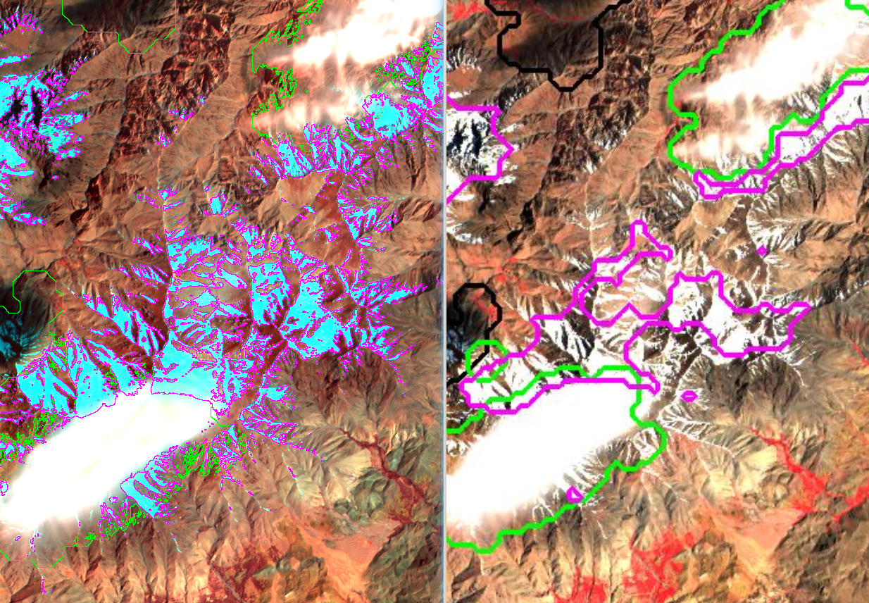
As an illustration we compare the original L2A cloud/snow masks computed at 200 m resolution to the new cloud/snow masks below:
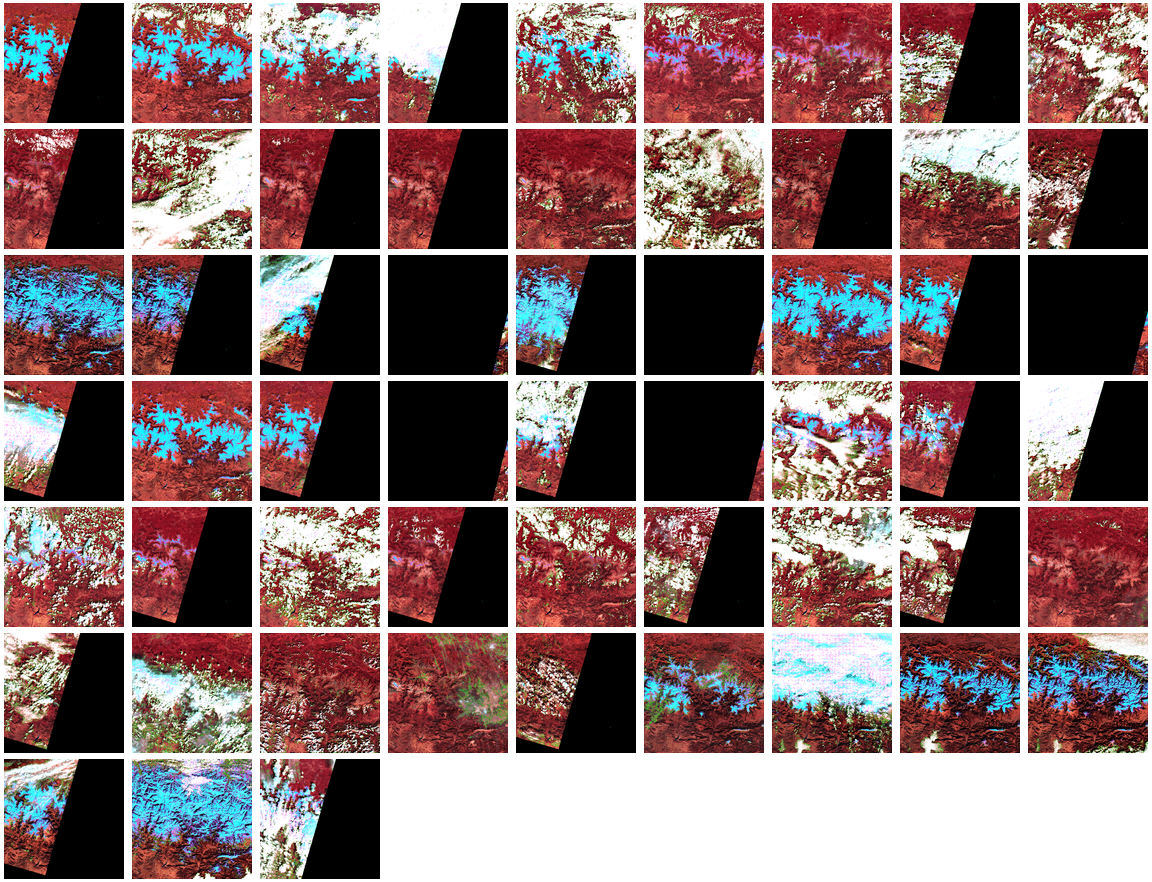
The LIS code was implemented in Python using OTB and GDAL librairies by Manuel Grizonnet at CNES and is compatible with SPOT4, Landsat-8 and Sentinel-2. We were able to run the code for a series of 57 Landsat-8 scenes over the Pyrenees available from THEIA in ~6 hours (tile D0005H0001). First tests with Sentinel-2A were also very promising but I will probably show this in another post! (I did: First Sentinel-2 snow map)
Ideally we would like to further validate LIS using terrestrial time lapse images in the next year. This could also allow a calibration of the parameters (e.g. $$N_2, R_2$$). However we feel that it does already a good job after a visual inspection of dozens of images in Morocco, Pyrenees, and the Alps. The next step will be to develop an interpolation method to provide a 5-day gap-filled snow product based on images from both Sentinel-2. Meanwhile, CNES is implementing the operational version on the MUSCATE ground segment, and we hope to start producing and distributing snow maps with Sentinel-2 in 2016, before the snow completely melts. Summer will be back. You can read a further example about this product here: State of the snow cover in the Pyrenees in January 2016. A more detailed documentation of the algorithm can be downloaded from the LIS project repository.